The method described in the original article basically assumes that adding a consequence and a probability together will yield a meaningful number. If we add the two numbers together, which do not have the same units of measure, the end result is meaningless. For example, would an electrician add the voltage and the amperage of an electrical motor to determine the wattage? (Hopefully not.) A strong caution about the use of distance methods for risk assessments is probably best stated by Edmund H. Conrow in his book, Effective Risk Management: Some Keys to Success:

"There are innumerable representations of risk possible, but most do not appear to have a convincing mathematical and probabilistic basis. Computation of risk should generally be performed using a simple multiplicative representation (P * C), assuming the underlying data do not violate any mathematical or probabilistic principle."²

Understanding risk is important for making sound business decisions. If the basis for understanding risk is flawed, then businesses are making decisions on flawed information. Unfortunately, the distance method (Euclidean distance or "positional risk") described to calculate risk represents a potentially poor understanding of risk, which could lead to making poor decisions. Prior to looking at an example of how distance methods could lead to poor business decisions, we will first look at risk.

What is Risk?

ISO 31000 and ISO 73 both define risk as the "effect of uncertainty on objectives."³ This broad definition encompasses: 1) Either a positive or negative effect, 2) Objectives that can reflect one or many different categories, such as safety, environmental, or financial goals, and 3) The uncertainty reflecting the likelihood (probability) of events actually occurring. This broad definition allows for qualitative, semi-quantitative, and quantitative risk analysis of the consequences and associated probabilities.⁴

Correspondingly, risk has been traditionally defined as the likelihood and the consequence of an event where the expected value of the risk is expressed mathematically as:

Risk = Consequence * Probability.⁵

I refer to this as traditional risk. This basic mathematical and probabilistic concept of risk is used for common industry tools, such as event tree analysis, fault tree analysis, Monte Carlo simulations and other tools. In addition, this definition of risk has been used in many industries (insurance, refining, medical research, statistics, banking, etc.) for many years. Furthermore, the mathematics supporting this method also allows cumulative risk to be calculated.⁶ Thus, we have strong reasons for using the traditional quantitative risk analysis.

Visual Representation of Risk

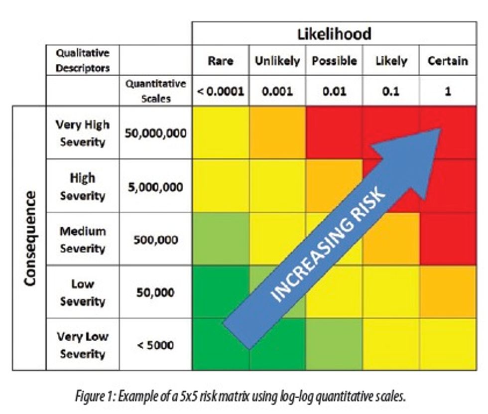
Since the positional risk in the original article was applied on a risk matrix, we should discuss risk matrices and how they illustrate risk. There are numerous methods and approaches for risk matrices.⁷ A risk matrix can often be developed where the probability and consequence axes have quantitative scales in conjunction with qualitative descriptors.⁸ The quantitative scales allow for the calculation of risk using the traditional C * P method, while visually representing the increasing levels of risk by color. An example of a risk matrix is shown in Figure 1. This example risk matrix utilizes qualitative descriptors, associated quantitative scales that have a log-log scale and a color scheme that reflects relative risk that is consistent with the calculated expected value of the risk.

Figure 1: Example of a 5x5 risk matrix using log-log quantitative scales.

Often, the quantitative scales will use a log-log scale to allow the risk matrix to represent a very wide spectrum of risk. Within some industries, risk matrices that have a range of four to five orders of magnitude are used on a daily basis. For consequences, the matrix could show the progression from a slight injury to a minor injury to a major injury to fatalities to multiple fatalities. For the probability, the matrix could showa 0.1% to a 1% to a 10% to a 100% probability that an event could occur within a year. It is important to keep in mind that risk matrices are typically not linear and represent exponential increases in magnitude along the axes. In general, risk matrices may vary by design, application and color coding, meaning we should be mindful of applying any generalizations.

Comparing Positional Risk to Traditional Risk Methods

To illustrate the difference between positional risk and traditional risk, we will compare constant risk as defined by each method. The visual representation of constant risk is similar to isolines (lines of constant elevation) on a contour map. Both conflicting definitions (traditional vs. positional) of risk can be represented by lines of constant risk, much like lines of constant elevation on a map. In a contour map, the elevation is set to a constant level and the lines represent the constant elevation using longitude and latitude as the axes. With risk, we can set the risk to be a constant level and chart the constant risk with consequence and probability axes.

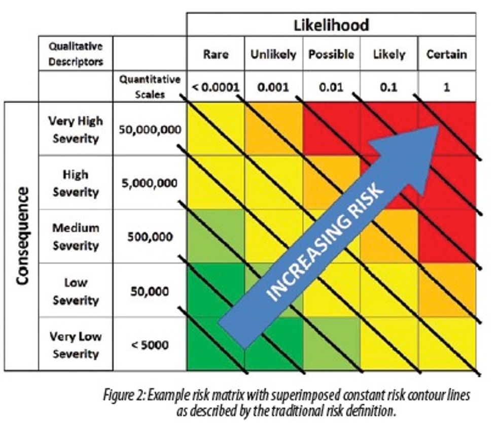
In the traditional risk definition, constant risk appears as straight lines on log-log scale charts (similar to many quantitative risk matrices). An example of constant risk lines using the traditional risk definition are illustrated on a risk matrix with a log-log quantitative scale shown in Figure 2. Also visible in Figure 2, the lines of constant risk run parallel, with the color changes representing increasing risk levels.

Figure 2: Example risk matrix with superimposed constant risk contour lines as described by the traditional risk definition.

In the distance method proposed (positional risk), the constant risk is a fixed distance from the origin point of the graph, which looks like concentric quarter circles. An example of constant risk lines using the positional risk method is shown in Figure 3.

Figure 3: Example risk matrix with superimposed constant risk contour lines as described by a distance method (“positional risk”) definition.

A problem becomes immediately clear with the positional risk in Figure 3, whereas the constant risk lines wander through several levels of differing risk. In Figure 3, the constant risk line starting in the upper left moves from yellow to orange to red and back again, which indicates that the risk is not nearly as constant as proposed.

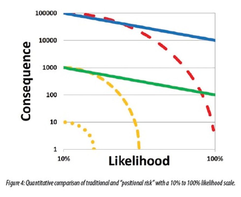
To further illustrate the difference between traditional risk and positional risk, we can compare the two methods, as shown in Figure 4. In the figure, we have superimposed two constant traditional risk lines withthree constant distance lines. The traditional risk is represented by two constant risk lines shown by the blue and green straight lines, while the positional risk is represented by the dashed lines. For the purpose of the example, we are using probabilities from 10% to 100% likelihood and consequences of $1 to $100,000, much like the risk matrix in Figure 1 but with reduced scales on the x-axis. In Figure 4, the perceived slope of the traditional constant risk lines, as compared to Figure 2, has changed due to the x-axis scale, but the underlying mathematics and actual values of the risk have not been affected by the change in scale.

Figure 4: Quantitative comparison of traditional and “positional risk” with a 10% to 100% likelihood scale.

Difference Between Risk Definitions

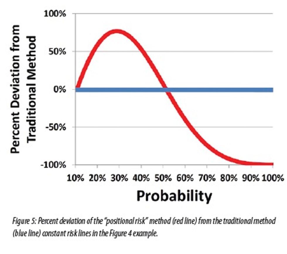
We can calculate the difference between the traditional risk calculation method and the positional risk method. First, we need a starting point where the two methods agree on the risk. This is a single point where the probability and consequence are the same for both methods, i.e. where lines intersect. In Figure 4, the solid blue line and the dashed red line intersect at a probability of 10% and a consequence of $100,000. By calculating the risk along the paths of the red and blue lines, the differences in risk level can be shown as a percent difference between the two. Figure 5 shows the calculated deviation between the traditional risk calculation method and the positional risk calculation method, which varies from +80% to -100% of the traditional method of evaluating the level of risk.

Figure 5: Percent deviation of the "positional risk" method (red line) from the traditional method (blue line) constant risk lines in the Figure 4 example.

Impact from Misunderstanding Risk Example

Given the magnitude of the deviation between the traditional risk and positional risk, we should look at how the difference of risk measurement could impact business decisions. Suppose we have a problem, Option A, within our hypothetical plant that has a 95% probability of occurring with a consequence of roughly $100. We can graphically represent this as arrow "A" in Figure 6. The length of arrow "A" shows the positional risk method for calculating risk. We also see the traditional definition of risk associated with the problem being shown as the green line.

To eliminate this problem, our hypothetical plant underwent an improvement effort to develop a solution. The proposed solution, Option B, resulted in changing the risk, as shown by arrow "B." Using the positional risk method, the risk of Option B was less than arrow "A" because the length of arrow "B" was shorter than arrow "A." If we had used the traditional risk method, we would have understood that both Option A (the original problem) and Option B (the proposed solution) have the same risk level as represented by the green line.

Figure 6: “Positional risk” incorrectly shows improvement from A to B, whereas actual risk has remained constant.

Thus, if we had used the positional risk in our risk assessment for our project screening and approval process, we would have approved and implemented a project that would not have reduced the overall risk of our hypothetical plant. With respect to the project, we would have had a negative return on our investment even though the positional risk clearly (and incorrectly) showed an improvement.

Conclusion

The use of Euclidean distance for comparing and assessing risk is not consistent with the mathematics used in other industry-accepted reliability and risk analysis methods. Without a solid understanding of the risk, we have incomplete information to make sound business decisions. ISO 73 and 31000 may allow for a broad range of risk analysis methods, but the practitioner should be mindful of the limitations of the methods, tools, underlying assumptions, limitations and objectives when using various methods to assess risk. Thus, caution should be used when using Euclidean distance or other distance methods when comparing risk as described in the original article.

References

^{1. Nelson, Terry, "Risk & Criticality, Understanding Potential Failure," Uptime magazine October/November 2011: 56-58.}

^{2. Conrow, Edmund H., Effective Risk Management: Some Keys to Success, Reston: American Institute of Aeronautics and Astronautics (AIAA), 2003, Page 232.}

^{3. International Standards Organization (various years), IEC/ISO 31010, ISO 31000 and ISO 73 publications, Geneva, Switzerland.}

^{4. International Standards Organization, ISO 31000, Geneva: 2009, Page 18.}

^{5. Fullwood, Ralph R., Probabilistic Safety Assessment in the Chemical and Nuclear Industries, Woburn: Butterworth-Heinemann, 1988, Page 6. Cox, Louis A., Risk Analysis of Complex and Uncertain Systems, New York: Springer Science, 2009, Page 108. Andrews, J. D. and Moss, T. R., Reliability and Risk Assessment, New York: The American Society of Mechanical Engineers, 2002, Page 9.}

^{6. Modarres, Mohammad, Kaminskiy, Mark and Krivtsov, Vasiliy, Reliability Engineering and Risk Analysis: A Practical Guide, New York: Marcel Dekker, 1999, Page 466.}

^{7. NASA, NASA Systems Engineering Handbook (NASA/SP-2007-6105,) Rev. 1, 2007, Page 145. Garvey, Paul R., Analytical Methods for Risk Management: A Systems Engineering Perspective, Boca Rotan: Chapman & Hall/CRC, 2009, Page 113. International Standards Organization, IEC/ISO 31010, Geneva: 2010, Pages 82-86.}

^{8. Barringer, H. Paul, Risk-Based Decisions, Sept. 8, 2009, http://www.barringer1.com/nov04prb.htm.}

Brian Y. Webster, CRE is currently the Reliability Manager for a refinery in Washington. He has more than 18 years of experience in the Oil and Gas Industry and served as an Ordnance Officer in the U.S. Army.

Read the response to this article by Terry Nelson - Risk Calculation Methodology