Biography
Timothy A. Dunton Vice President Product Development
Born and Educated in the UK, Tim spent 14 years with Shell Tankers UK. Ltd. as a marine engineer, serving on Oil and LNG tankers in a variety of positions including Cargo Engineer. After emigrating to Canada Tim brought his practical experience to IRD Mechanalysis as a Consulting Service Engineer, providing training, software support and on site analysis services throughout Canada.
In 1991 Tim joined Update International as a senior instructor where he conducted various vibration and skills related courses in both the public and in-plant arenas throughout the world. During his tenure at Update Tim assisted in development of several seminars in the subjects of vibration analysis, machinery skills and bearings. Tim was also responsible for upgrading several seminars and developing award winning multimedia interactive software. Tim is a regular speaker at various maintenance conferences throughout the world. Now with Universal Technologies, Tim's primary responsibility is in the area of multimedia product development but he continues to be active in the teaching arena.
Introduction
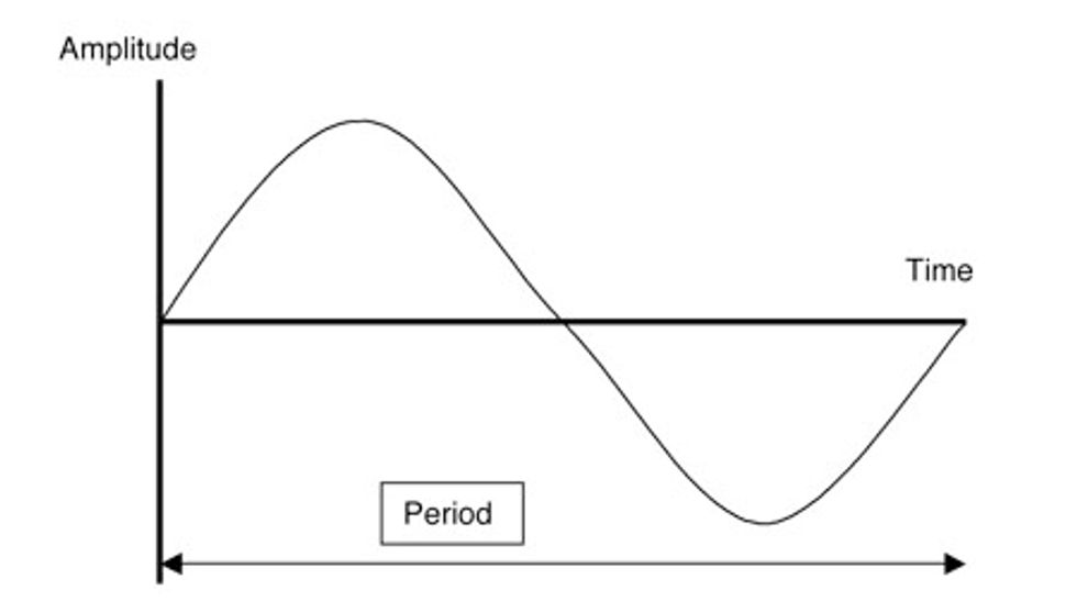
The analysis of time waveform data is not a new technique. In the early days of vibration analysis time waveform data was viewed on oscilloscopes and frequency components calculated by hand. The relationship between frequency and time is as follows:
f = 1/p
where: f is the frequency in Hz p is the period in seconds (the amount of time required to complete 1 cycle)

Knowledge of this relationship permits the determination of frequency components from the raw waveform data.
For example:

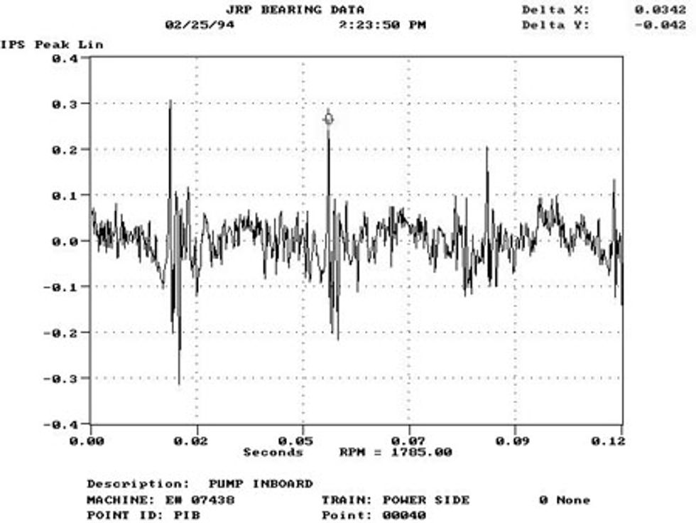
The above waveform was acquired from a 1785 RPM pump. The time spacing between the impacts is 0.0337 seconds. From this information the frequency can be determined.
f=1/p = 1/0.0337 = 29.67Hz = 1780CPM
This indicates that the impact is occurring at a frequency of 1 x RPM.
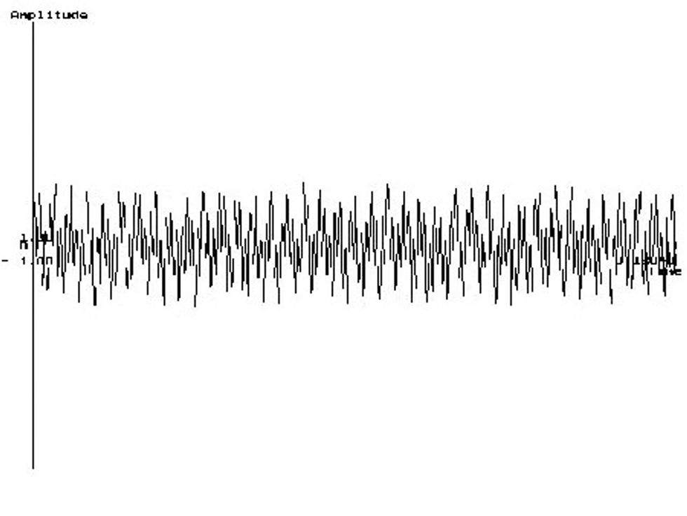
In most situations the time waveform pattern is very complex as illustrated below and therefore the determination of frequency components is extremely difficult using this method and is not recommended.
In most situations time waveform data is best utilized by applying the principles of pattern recognition and if necessary calculating the frequency components of the major events in the waveform pattern.
When to Use Time Waveform
Time waveform can be used effectively to enhance spectral information in the following applications:
- Low speed applications (less than 100 RPM).
- Indication of true amplitude in situations where impacts occur such as assessment of rolling element bearing defect severity.
- Sleeve bearing machines with X-Y probes (2 channel orbit analysis)
When NOT to Use Time Waveform
Time waveform can be applied to any vibration problem. In some situations normal spectral and phase data provide better indications as to the source of the problem without the added complexity of time waveform data. Examples include:
- Unbalance on normal speed machines
- Misalignment on normal speed machines
Instrument Setup for Time Waveform
The key to successful analysis of time waveform data is in the set up of the instrument. The following items have to be considered when setting up the instrument
Units of Measurement
Amplitude measurement units should be generally selected based upon the frequencies of interest. The plots below illustrate how measurement unit selection affects the data displayed. Each plot contains 3 separate frequency components of 60Hz, 300Hz, and 950 Hz.
This data was taken using displacement note how the lower frequency at 60 Hz is accentuated.
The same data is now displayed using velocity note how the 300Hz component is more apparent.
The same data is now displayed using acceleration note how the large lower frequency component is diminished and the higher frequency component accentuated.
The unit of measurement displayed in time waveform data should be the natural unit of the transducer used. For example if a displacement reading is required, then a displacement transducer should be used. In most cases where modern data collectors are employed this means that acceleration will be the unit of choice. If data is gathered from non-contact probes on sleeve bearing machines displacement is usually used.
Time Period Sampled
For most analysis work the instrument should be set up to see 6-10 revolutions of the shaft being measured. The total sample period desired can be calculated by this formula
Total sample period [seconds] = 60 x # of revolutions / desired RPM
The following table Illustrates common time period in seconds by machine speed
| Machine RPM | Time period for 6 revolutions (secs.) | Time period for 10 revolutions (secs.) |
| 3600 | 0.1 | 0.167 |
| 1800 | 0.2 | 0.333 |
| 1200 | 0.3 | 0.5 |
| 900 | 0.4 | 0.667 |
| 300 | 1.2 | 2.0 |
| 100 | 3.6 | 6.0 |
Some instruments do not permit the setting of time period data when acquiring time waveform data. With these instruments it is necessary to set an equivalent FMAX setting. The appropriate FMAX setting can be calculated by the following formula
FMAX [CPM] = Lines of Resolution x RPM / # of Revolutions desired
The following table Illustrates the common FMAX settings for 1600 lines of resolution by machine RPM
| Machine RPM | FMAX for 6 revolutions | FMAX for 10 revolutions |
| 3600 | 960kCPM | 576kCPM |
| 1800 | 480kCPM | 288kCPM |
| 1200 | 320kCPM | 192kCPM |
| 900 | 240kCPM | 144kCPM |
| 300 | 80kCPM | 48kCPM |
| 100 | 26kCPM | 16kCPM |
Resolution
For time waveform analysis it is recommended that 1600 lines (4096 samples are used). This ensures that the data collected has sufficient accuracy and key events are captured.
Averaging
In most data collectors averaging is performed during the FFT process. Unless synchronous time averaging is invoked the time waveform presented on the screen will be the last average taken even if multiple averages are selected in the instrument setup. It is normal therefore to take a single average. Overlap averaging should be disabled. Synchronous time averaging can be used to "synchronize" data acquisition to a particular shaft. This can be useful on gears where broken teeth are suspected to assist in the location of the defective teeth relative to a reference mark. It is also useful on reciprocating equipment to "time" events to a particular crank angle.
Windows
Various windows can be applied to the time waveform prior to performing the FFT. The purpose of these windows is to shape the spectrum and minimize leakage errors. Some instruments can apply these windows to time waveform data as well. This would force the data to zero at the start and end of the time sample potentially losing data. To eliminate this effect a uniform or rectangular window should be applied.
Interpretation of Waveform Data
Unbalance

The classic sine wave illustrated above is rarely seen in acceleration time waveform. This is because acceleration emphasizes the higher frequency components that are almost always present in the vibration signal. This de-emphasizes the underlying lower frequency signal.
The waveform below is more representative of sinusoidal vibration when viewed in acceleration. Note the high frequency components superimposed on the lower frequency.
Misalignment
Although the classic symptoms of misalignment are M and W shapes in the time waveform, these symptoms cannot be relied upon. The relative phase angle between the 1 x RPM and 2 x RPM components determines the shape or pattern of the plot.
The pattern above illustrates the classic pattern of misalignment. In the pattern below the relative phase between 1 x RPM and 2 x RPM was changed 90 degrees resulting in a very different pattern.
The pattern below originates when the 1 x, & 2 x, vibrations are 0 degrees apart.
Amplitude Symmetry
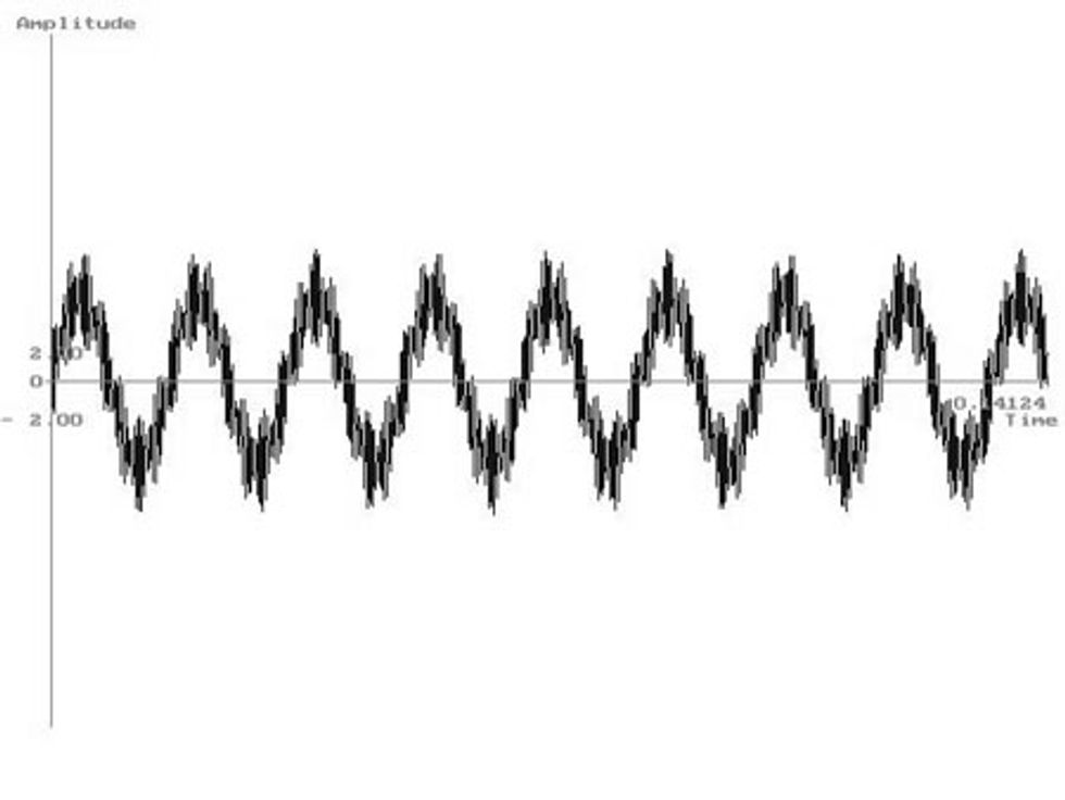
When observing time waveform data symmetry above and below the centerline axis is important. Symmetrical data indicates that the machine motion is even on each side of the center position. Non symmetrical time waveform data indicates the motion is constrained possibly by misalignment, or rubs.
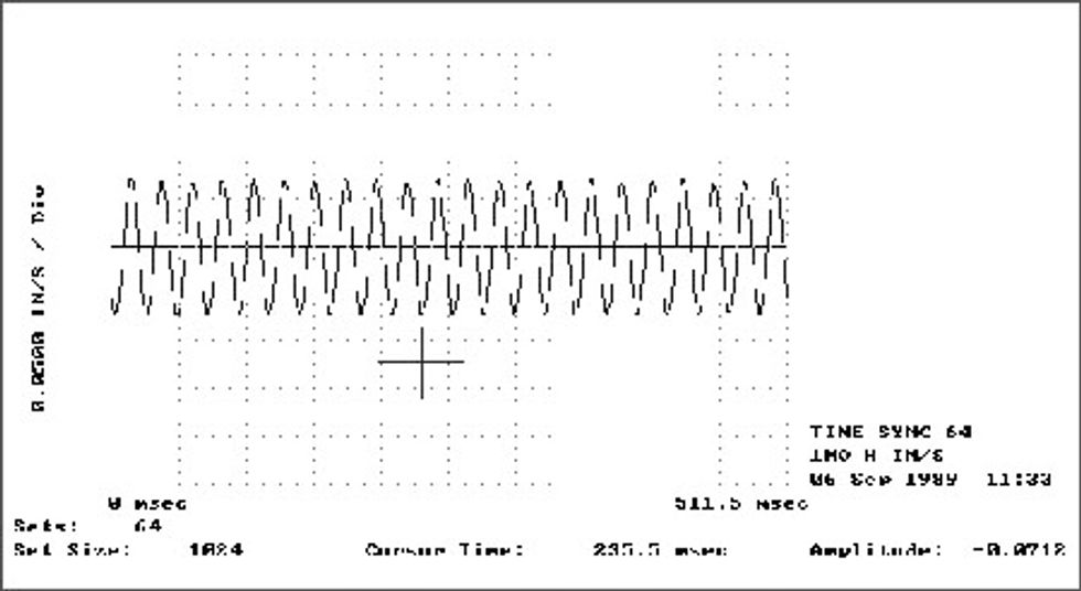
This waveform pattern is symmetrical above and below the zero line.
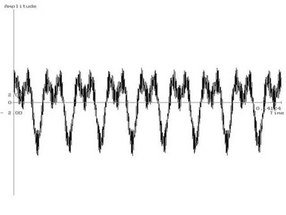
The following waveform pattern is non-symmetrical above and below the zero line. The amplitudes below the line are significantly higher than those above the line. In this case a misalignment condition was the source. The markers on the plot indicate 1 x RPM.
Symmetry of the Time Axis
When the previous time waveform is observed with 1 x RPM markers present it can be noted that the waveform pattern although complex is repetitive with 1 x RPM. This indicates that the vibration is synchronous to RPM.
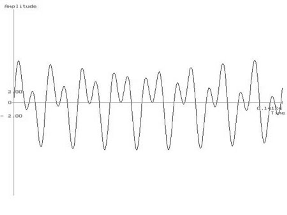
The waveform pattern below indicates a non-repetitive pattern characteristic of non- synchronous vibration.
This example, is of two frequency sources that are not harmonically related. (58 Hz and 120 Hz) This is the kind of signal that could be created when a 2 pole motor has an electrical hum problem.
Higher frequency component "Riding" on other wave
It can be seen that the higher frequency wave does not always start at the same part of the lower frequency cycle and therefore appears to "ride" on the other wave causing symmetry to be lost.
Care must be exercised when determining symmetry of the time axis. 1 x RPM markers are available in most software programs and should be used to avoid confusion.

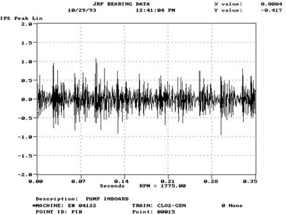
At first glance this waveform appears to have large impacts occurring with somewhat similar spacing. The horizontal axis is scaled in time units.
By using RPM as the horizontal axis and applying 1 x RPM markers the major impacts can be seen to be occurring at approximately the same part of the revolution. However closer inspection reveals that the spacing is not exactly synchronous In this case the problem was a single large defect on the inner race of a bearing. the change in amplitude of the defect was due to the defect coming in and out of the load zone
This is the FFT taken from the above machine note the highest amplitude at BPFI is< 0.05 ips !
(15g pk @ BPFI = 2.13 ips)
Beats & Modulation effects
Another excellent application for time waveform is the observation of beat frequencies and modulation effects. Often these phenomena are audible. The time span for data collection should be set to capture 4-5 cycles of the beat.
The time period between the beats on the above waveform is 0.5 s. From this information the frequency of the beat is calculated at 120 CPM. This represents the frequency difference between the two source frequencies In this case the beat was caused by interaction between a 2 X RPM vibration source and a 2 x fL vibration source on an induction motor.
Impacts
When the FFT process is applied to a signal that contains impacts the true amplitude of the vibration is often greatly diminished. The following time waveform was taken from an 1800 RPM machine. It shows several random impacts with magnitudes over 6 g pk. The cause of this signal was a failed rolling element bearing. The shape of the waveform often appears to be a large spike followed by a "ring down".
The plot below was a velocity spectrum taken from the same bearing note the amplitude of vibration is less than 0.04 ips!
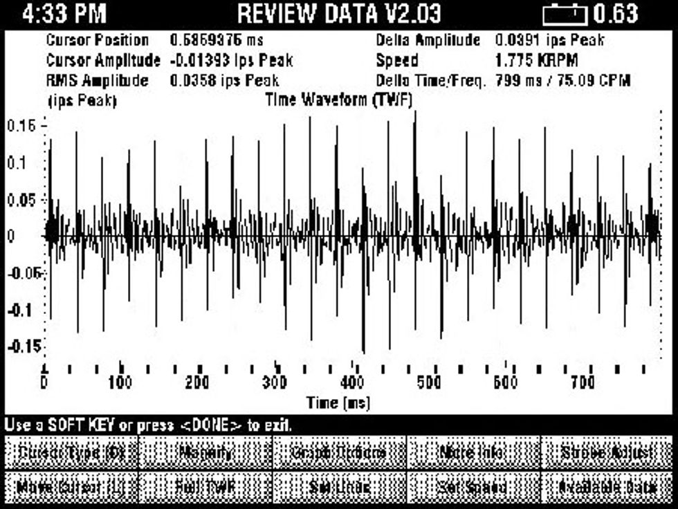
Care must be exercised when assessing the amplitude severity of 1 x RPM impact vibration using spectrum. This is the spectrum of a machine with where the key is impacting the coupling guard. The amplitude scale indicates amplitudes of less than 0.02 ips.
This is the time waveform from the above machine the amplitude of the impacts exceeds 0.15 ips.
In this case severe damage had occurred to the key and shaft of the machine in question.
Conclusions
In conclusion, how is this information practically applied in a condition based maintenance program?
- Time waveform analysis is an analysis tool. The writer would not recommended that it be taken on all measurement locations on a regular basis. This would add significantly to the time required and data storage requirements.
- Use Time waveform for the following selected analysis situations to enhance FFT information
- Low speed applications (less than 100 RPM).
- Indication of true amplitude in situations where impacts occur such a assessment of rolling element bearing defect severity.
- Gears.
- Sleeve bearing machines with X-Y probes (2 channel orbit analysis
- Looseness.
- Rubs.
- Beats
- Impacts
- Use an appropriate measurement unit
- Rolling element bearings, gears, looseness, rubs, impacts ...acceleration
- Sleeve bearing machine with x-y probes...displacement
- Initially set up to observe 6 -10 revolutions of the shaft in question
- Study the following symptoms in the waveform
- Amplitude
- Amplitude Symmetry
- Time Symmetry (use RPM markers)
- Beats / Modulation
- Impacts (shape and amplitude)
Remember use time waveform to ENHANCE not REPLACE spectral data.
Author: Timothy A Dunton, Reliability Solutions LLC