Plant and refinery problems require accurate measurements to assess plant productivity and reliability. In fact, as management guru Peter Drucker stated, “You can’t manage what you can’t measure,” forms the basis to many real-world problems, from engineering optimization studies to troubleshooting plant machinery and equipment. Drucker’s statement also alludes to the fact that you cannot know whether or not you are successful unless success is defined and tracked.

This case study concerns itself with a problem that many operating plants and refineries may be facing as a result of standardization, optimization of cost versus design, or simply older construction and the nature of refinery design. It also reflects on the value of utilizing process engineering tools to help address issues with machinery monitoring, reliability and troubleshooting.

The Problem

The problem at hand concerns a centrifugal API 610 between bearing (BB) pump in heavy vacuum gas oil (HVGO) service. The pump’s datasheet provides all the relevant information connected to the maximum, minimum and rated operating conditions. As a result of various concerns, particularly connected to pipe strains and thermal wrapping of the pump’s casing during commissioning, the original equipment manufacturer (OEM) requested the clearances of the pump to be opened up due to seizure of the pump on start-up. Once the clearances were opened, this introduced additional hydraulic instabilities in the pump, adding to an already reduced seal mean time between failures (MTBF).

The Challenge

The challenge in this case was connected to accurately being able to monitor and measure pump performance and hydraulic dynamics to understand what exactly was going on during machinery operation. Plants typically monitor flow; as per API 610, the preferred operating margin for a centrifugal pump is between 70 and 120 percent of the pump’s best efficiency point (BEP) during pump operation. However, not many plants monitor the actual head the pump generates during operation. Part of this situation is complicated by the fact that many older plants and even some new plants do not have the necessary instrumentation, such as suction pressure transmitters mounted on the inlet of the pump or discharge instrumentation mounted on common headers, leading to issues of accurately understanding pump operation. Often, this leads to a standstill situation in a live plant when it comes to understanding, measuring and troubleshooting machinery. Usually, multiple iterations need to be done, costing time and resources to diagnose a problem with a given asset.

This case study presents one way to address the challenge of lacking instrumentation by utilizing other process variables, establishing a direct link to the pump’s parameters (suction pressure in this case) and then working along to develop a model to monitor and measure machinery performance without additional cost and resource utilization.

Calculation

Basic process engineering fundamentals can be utilized to model process flow around the pumps in operation. This is done by mapping the head versus flow on the pump’s performance curve.

Total discharge head (TDH) of the pump is computed by:

(Equation 1)

Where:
   TDH: Total discharge head in meters (m)
   Hdischarg: Discharge head (m)
   Hsuction: Suction head (m)
   Hfriction: Friction loss (m)

TDH is a representation of the ability of the pump to both meet the system’s requirement at a given flow and overcome pressure drops. Equation 1 is the summation of the static head with the friction loss head. The static head is the difference between the discharge head and the static head. Friction loss represents the pressure drops across the pipe and fittings; it can be represented by Darcy’s law.

(Equation 2)

Where:
   f: Friction factor
   L: Length (m)
   v: Fluid velocity in meter per second (m/s)
   D: Internal diameter (m)
   g: Standard gravity (m/s2)

It is a factor of the length of the pipe, the diameter of the pipe and the friction factor based on the velocity across the pipe, as seen in Equation 2.

In the simple case where pressure transmitters are installed on both the suction and discharge line, Equation 1 can be used to calculate the TDH. In this case, it is possible to calculate both the discharge and suction head given that you know the specific gravity of the fluid using Equation 3 to convert the pressure readings into head.

(Equation 3)

Where:

H: Head (m)
P: Pressure (suction/discharge) (Kpa)
SG: Specific gravity in kilogram per meter (kg/m ³)
g: Standard gravity (m/s ²)

In some instances, there is a pressure transmitter on the suction line, in others, on the discharge line (a more frequent scenario) and in some older plant installations, there is a possibility that there are no transmitters located on the suction line and a pressure transmitter located on a common header that is being fed by multiple pumps.

Case 1

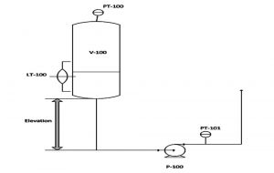
Figure 1: Pumping system flow diagram with no pressure transmitter on suction side

A scenario with only a pressure transmitter on the discharge line is illustrated in Figure 1. Vessel V-100 is connected to pump P-100. Also in Figure 1, a pressure transmitter, PT-101, is on the discharge side of the pump, but there is none on the suction side. It is possible to calculate the suction head using the pressure measured by PT-100 (pressure inside V-100) and LT-100 (liquid level inside V-100), factoring in the friction loss or piping loss and adding the elevation between V-100 and P-100, as shown in Equation 4.

(Equation 4)

Where:
   Hs: Suction head (m)
   Pv: Vessel pressure (KPag)
   SG: Specific gravity (kg/m3)
   g: Standard gravity (m/s2)
   Lv: Liquid level inside the vessel (m)
   h: Elevation (m)

Using PT-101, the discharge head is:

(Equation 5)

Where:
   HD: Discharge head (m)
   PD: Vessel pressure (KPag)
   SG: Specific gravity (kg/m3)
   g: Standard gravity (m/s2)

Combining Equations 4 and 5:

(Equation 6)

Case 2

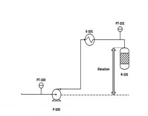
Figure 2: System flow diagram with no pressure transmitter on discharge side

Figure 2 illustrates a scenario with a pressure transmitter on the suction line of the pump, but not on the discharge line. Process fluid is being pumped by P-100 toward E-101, where it is heated before being sent to the reactor R-101. The pressure transmitter PT-101, located at the entrance of the reactor, can be used to calculate the discharge head of the pump, as shown in Equation 7. The discharge head is a factor of the elevation between the center line of the pump and the pressure transmitter, as well as the pressure drop across the pipes, as well as E-101.

(Equation 7)

Given PT-100 on the suction line, the suction head can be calculated:

(Equation 8)

Where:
   Ps: Suction pressure (Kpa)

Combining Equations 7 and 8:

(Equation 9)

Case 3

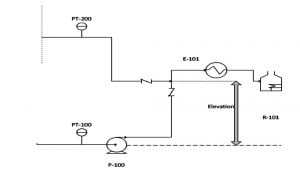
Figure 3: System flow diagram with no pressure transmitter on discharge side

Figure 3 is somewhat similar to the scenario mentioned in Case 2, where there is no pressure transmitter on the discharge line of the pump. The difference is with the location of pressure transmitter PT-200, which is on a different stream in a different area and is combined with the discharge stream of P-100 before being sent to E-101.

Case 4

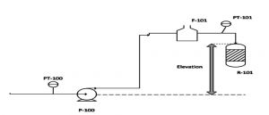
Figure 4: System flow diagram with no pressure transmitter on the discharge of a pump

Another scenario is where there is no pressure transmitter on the discharge line, as illustrated in Figure 4. In this system, a fluid is being pumped to furnace F-101 before being sent to the reactor R-101. On the suction side, PT-100 provides the pressure reading, while on the discharge side of the pump, a pressure transmitter is not installed. Therefore, you have to calculate pressure on the discharge using PT-101. Since the pressure transmitter is located after the furnace, the process fluid is a two-phase mixture. Therefore, it is not possible to apply Darcy’s Law (Equation 2), which only applies to liquids. Empirical models based on either homogeneous models or nonhomogeneous models, such as the methods used by Friedel, Lockhart and Martinelli ¹, can be used to calculate the piping losses. These calculations are out of the scope of this paper, however, a reference link is provided for further reading.

Value of Generating Real Time Head Flow Curves

A lot of valuable pump operation data can be gathered from monitoring real-time performance of the pump. Typical points to consider during analysis, troubleshooting and performance of the machinery include:

1. If the pump is generating lesser head than the original curve, this can point toward issues connected to mechanical wearing of the pump’s components, recirculation and other performance degradation effects, such as opening up of the pump’s clearances.
2. It is relatively easy to ascertain hydraulic issues by comparing the operating performance of the pump. This includes incorrect impeller trims, vibration-related issues and off margin operation from the best efficiency point (BEP).
3. Speed changes; if the pump is running off a variable frequency drive or turbine drive, then speed changes can be correlated to an increase or decrease in the head being generated by the pump in real time.
4. Process-related fluctuation can be determined indirectly by seeing a time varying trend on the head versus flow curve.
5. Trending of motor amperage on the performance curve can provide valuable information on impeller sizes and other hydraulic factors that are specific to the pump. High flow impellers would draw more energy than low flow impellers.
6. Pump rerating can be better addressed when real-time pump operating can be understood. This helps in minimizing underrating and overrating of newly rated pumps and ensures better operational reliability.

Conclusion

In any operating plant, consideration should be given to utilizing process engineering tools and, in the absence of relevant instrumentation, real-time equipment monitoring should be encouraged. Plant deficiencies, such as a lack of instrumentation, should not impede cost-effective ways to improvise on existing problems.

Process modeling simulation software can be utilized in conjunction with rotating equipment problems to address, monitor and troubleshoot issues that would otherwise require a reactive approach, like shutting down equipment and impacting production downtime. While calculations and analysis in a running plant should be kept to a minimum to address problems on a fast and efficient basis, accurate modeling and an understanding of the process surrounding any rotating equipment is critical in helping to improve reliability.

Reference

1. http://ltcm.epfl.ch/files/content/sites/ltcm/files/shared/import/migration/COURSES/TwoPhaseFlowsAndHeatTransfer/lectures/Chapter_13_PART_1.pdf