Problems with reliability appeared with the beginning of human activity. However, the ways of solving these problems were different and they were changing with growing complexity of technical systems. The retrospective view shows that the way of solving reliability problems depends on the ratio between the complexity of the system and the ability of people to obtain information about the system and its elements.

For example, it is not difficult these days to find out if a crowbar is reliable enough to do a particular job. The ability of modern modeling packages is sufficient enough to simulate load and stress distribution along the bar. Non-destructive testing methods are sufficient for proving the absence of hidden cracks or voids in the metal structure. Why is this important? It means that if you have an accurate, physical model of the object and sufficient information about the current condition of the object, you can accurately predict what is going to happen to the object.

Many diagnostic methods have been developed and many reliability models have been created, so why does reliability remain a problem?

What Is Reliability and Why Is It a Problem?

Let’s start from the question: Which system would you consider reliable:

• The one that would work for 100 hours;
• The one that would work for 1,000 hours;
• The one that would work for 10,000 hours?

Most people familiar with the reliability assessment would choose the one that would work for 10,000 hours because this is the most common understanding of reliability – the ability to work for a longer time.

But, what if it is a torpedo generator? The required operation time for it, before the torpedo hits the target, is several minutes. Will 100 hours be sufficient in this case? It certainly will. The opposite case is a valve for an artificial heart. It should be designed to work for at least 50 years, so even 10,000 hours wouldn’t be enough to call this system reliable.

So, all the system choices mentioned are equally unreliable if they failed unexpectedly. Considering the two examples, calling a system reliable would mean it works as long as expected.

Returning to the crowbar example, when you are able to get exhaustive information about the system, its behavior becomes completely predictable and you can call the system reliable.

Looking at reliability from the position of information, the complexity of technical systems were always ahead of the level of knowledge about these systems. In other words, there was always not enough information to determine time to failure accurately. Figure 1 shows the changes in the complexity of technical systems and, according, changes in the approach to reliability problems.

Figure 1: Change of approach to reliability problems with growing complexity of technical systems

As the Figure 1 diagram shows, for primitive systems and very little knowledge about them, there was an intuitive approach to reliability by go/no go tests. The failure could happen any time with the same probability.

The development of basic technical systems, such as a carriage, mill, hut, etc., required some basic knowledge that was mainly gained by experience, with some simple empirical modeling. This was better than nothing, but didn’t do much for the improvement of reliability.

The next period contained complex technical systems that presumed complex physical models. Calculations were more accurate, the modeling was more sophisticated and, as a result, reliability could be controlled to a certain degree. But, the knowledge was still not exhaustive, so to achieve higher reliability, the reserve factors were widely used. This method was acceptable before complex mobile systems were developed.

For example, one can improve the reliability of a shaft simply by increasing its diameter. However, it will increase its weight, too. While you can afford it for some stationary equipment, increased weight is always in contradiction with the restriction of mobile systems, which you are always trying to make lighter. Contradiction initiated the probability-based approach to reliability problems. A probability-based approach is, in fact, a compromise between the level of knowledge one has about a system and the safety factor you can afford.

The first electronic devices, with thousands of similar elements in their circuits, initiated a statistical approach. This gave very accurate results similar to physics, where a chaotic motion of molecules in gas creates determined pressure.

The problem was that the good results achieved in electronics stimulated scientists to apply the same principles to electrical engineering and, in particular, electrical machine manufacturing. But, because electrical machines don’t have thousands of similar elements, the theory was applied instead to mass production, where one is dealing with thousands of similar machines.

Although the approach works for manufacturers of high quantities of similar products, it doesn’t make the user happy. For example, if a machine fails, the user is not interested in hearing that it was one of 1,000 machines that were manufactured and all other 999 machines are working fine. To make sure every machine is reliable, enough information is required about the strength of the machine, as well as the stress an individual machine will be subject to. All this is considered information.

Reliability and Information

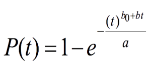
It is relatively easy to show mathematically that there is a direct relation between information and reliability. Take the Weibull distribution in its most applicable form for reliability:

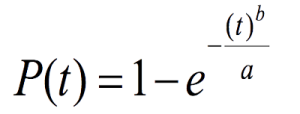
(Equation 1)

P(t) = probability of failure; a = scale parameter; b = shape parameter; t=time

The mean value [M( χ)] is:

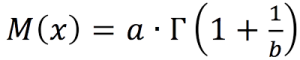
(Equation 2)

Γ = gamma function

The standard deviation [σ( χ)] is:

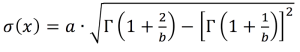
(Equation 3)

The per unit deviation is:

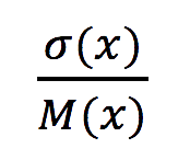
(Equation 4)

From these equations, you can see that the per unit deviation doesn’t depend on the scale parameter. It only depends on the shape parameter.

It is impossible to analytically find the shape parameter for each given per unit variation, however, Figure 2 shows how it looks graphically.

Figure 2: Shape coefficient of Weibull distribution as a function of per unit variation

As Figure 2 shows, the lower the variation, the higher the shape parameter. In technical terms, lower variation can be achieved by measuring and monitoring. And what is measuring and monitoring? Yes, it is gathering information.

Drawing a parallel with time-to-failure, you could say that if you know the strength of the element and the stress this element is subject to, then you will know if the element is going to fail during a given time period. And, the more accurate your information is, the more accurate the answer will be on whether it is going to fail or not.

This means the shape parameter of the Weibull distribution is a measure of information about the process or object. Taking this approach, one can modify the Weibull distribution as:

(Equation 5)

t= time;b₀ = initial information about the object (measuring); bt = information gathered during the time t (monitoring)

Expressing the failure rate [ λ(t)] from Equation 5, give the following:

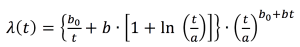
(Equation 6)

Now, have a look at the graph of this function, as shown in Figure 3.

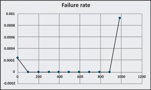
Figure 3: Failure rate curve received from modified Weibull formula

It looks like a classic reliability bathtub curve. Interestingly enough, this shape only can be achieved by a very specific combination of modified Weibull parameters. The curve shape is very sensitive to shape parameter which, as you already know, is representing the amount of information that you have about the object.

Using the Equation 6 with different parameters, you can simulate various scenarios. For example, if b₀ = 1 and b = 0, you get exponential distribution. Failure rate for this distribution is constant and depends on mean life expectancy. But, what does it mean from an information point of view? It means you only have some initial information. For example, you have a running motor; this is your initial information. You don’t know how long the motor was running before, the load, temperature, vibration, etc. As such, the failure can happen at any time and it becomes a Poisson process with a constant failure rate.

Is it possible to control reliability using information? Yes, here is an example.

An induction motor is driving a fan through the pulley and a set of V-belts. The drive end (DE) bearing is a 6305. The other parameters are as follows:

Basic dynamic load rating C = 22500 N;

Mean value of the dynamic load P = 1000 N;

Rotation speed n = 1500 RPM;

Belt tension force Pb = 400 N; force variation from 100 to 700 N

Magnetic pull force Pm = 150 N; force variation from 0 to 300 N

All other components (e.g., fan load, contact angle of the bearing, temperature, lubrication characteristics, etc.) are stable.

Assume a Gaussian distribution for the simplicity of the analysis.

1. Variation of the tension force: 700-100 = 600 N
2. Estimation of the standard deviation: 600/6 = 100 N
3. Variation of the magnetic pull: 300-0 = 300 N
4. Estimation of standard deviation: 300/6 = 50 N
5. Resultant variation: = 111.8 N
6. Estimated mean life expectancy according to the Lundberg-Palmgren model:
   = 10⁶/60/1500*(22500/1000)^3 = 12656 h
7. Standard deviation in per load units: 111.8/1000 = 0.1118
8. Sensitivity of the time to failure to the variation of the load: S = 3
9. Deviation of the time to failure because of the load variation: 3*0.1118 = 0.3354
10. Deviation of the time to failure in hours: 12656*0.3354 = 4245 h
11. Normalize value of the Gaussian distribution for 4,000 hours of operation: t = (12656-4000)/4245 = 2.039
12. Value of Ф(t) for the above t (from Gaussian distribution table): 0.472
13. Probability of failure within 4,000 hours: 0.5-0.472 = 0.028

If you monitor the belt tension and keep it at 400 N, the variation of the Pb would be 0. Substituting 0 in the above calculation gives the probability of failure:

P(T) = 0.000003

This example shows that by stabilizing only one parameter, one can increase the reliability of the system by 100 times.

Now that you know you can accurately predict the behavior of an object by having full information about it, the next issue is: do you need this information? The answer brings up another aspect of reliability: maintenance strategy.

Reliability and Maintenance Strategies

All maintenance strategies are about one question: Should you stop it or let it run? Two basic strategies are easy and give straight answer to this question. Reactive maintenance says run and face the consequences. Preventive maintenance says stop and absorb the cost. There are no questions about information for these two strategies. The only information preventive maintenance needs is the recommended time between maintenance.

The third real maintenance strategy is predictive. This is where you really need information to make a decision on whether to stop it or keep it running. Other strategies are a combination of predictive, with either root cause analysis (proactive) or failure mode and effects analysis (reliability-centered maintenance).

The latest, asset management, is not a strategy, but rather a facilitator for choosing and implementing the first three.

The most interesting option is definitely the predictive maintenance strategy. This is the one that requires informative answers to the question: should you stop it or let it run? As previously noted, you can achieve high reliability by determining the stress and strength of the machine very accurately. The main challenge is how accurate? You can perform a set of tests while the machine is running. This will give you b or the amount of information. If you know M(x), the mean value, then you can determine a and P(t) using Equations #2 and #5. Knowing P(t) gives you an estimation of possible losses as:

(Equation 7)

L = possible losses; T = time to repair/replace; C = cost of lost production per hour; C_r = cost of repair/replace

If estimated losses are higher than the cost of diagnostics performed to receive the given value of P(t), then you can increase the number of tests, making sure that they affect the b value.

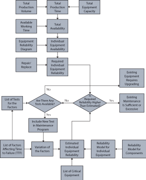
Figure 4: Block diagram of predictive maintenance planning

The diagram in Figure 4 shows a proposed algorithm for working out the number of tests required to achieve a certain level of availability. This diagram and the approach previously described provide the ways to further development in reliability improvement. The obvious challenges are:

• Developing more accurate mathematical models by connecting operational characteristics of equipment and their design parameters to time to failure;
• Improving quality of information provided by condition monitoring;
• Developing new ways for obtaining the information, preferably using online methods;
• Further development of the proposed model that connects the amount of information to reliability of the particular object.